Data Profiler & synthetic-data unite to overcome challenges
Integration solutions: Bridging data profiling and synthetic data
In the world of engineering and building models, the hurdles that exist to get a deliverable over the finish-line are known all too well. The first big hurdle may be answering a plethora of ad hoc questions: What’s in your data? Are there missing values? How is this data distributed? A better approach is a standardized library for answering questions like these above.
Capital One built Data Profiler—an open source project that performs statistical summarization and sensitive data detection on a wide range of data types. Data Profiler is now Capital One’s most starred open source repository. Data access and environment controls are vital to security, but they can also add inefficiencies to the testing and development life cycle. Workflows that use automated profiling and synthetic data can alleviate those inefficiencies by minimizing the need for access controls on the use of synthetic data in particular environments.
This is where synthetic-data, another Capital One open source library, comes into play. As my colleague described in a post, “Why you don’t necessarily need data”, the synthetic-data repository is a tool to generate artificial data that contains the same schema and similar statistical properties as its “real” counterpart.
Data integration benefits
The benefits of synthetic datasets are becoming more apparent—especially in financial services where the datasets need to be protected and access-controlled stringently. With synthetic data, however:
-
Data sharing can be quicker and safer—allowing for faster iterations of ideas and quicker testing of hypotheses.
-
Secure what needs to be and share what can be—keep the sensitive data locked down and share what can be without impediments.
How might you use these together in a seamless way? I’m glad you asked! Our team recently deployed an integration between these two libraries—creating a seamless experience between them using only 6 lines of code!
Understanding the workflow and process
Before jumping into the code of this integration, let’s first understand the flow of the process.
There are 4 stages to this process:
-
Load data: Read in the original dataset with dp.Data()
-
Profile data: Process the original data and generate a profile of the original data with dp.Profiler()
-
Initialize generator: Initialize the generator for generating the synthetic data
-
Generate synthetic data: Use the generator’s .synthesize() method
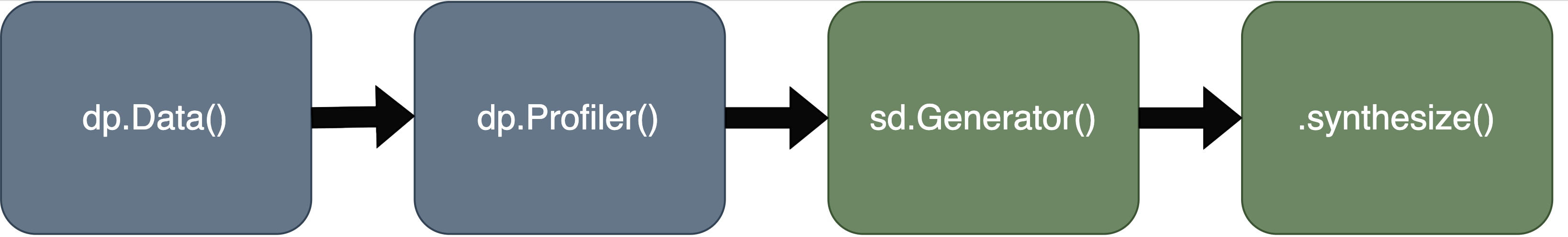
Process code example: dp.Data() ➞ dp.Profiler() ➞ sd.Generator() ➞ .synthesize()
Let’s take a look at the components of this workflow and how you can use profiling with synthetic generators.
Using Data Profiler
We use a dataset from the testing suite of synthetic-data. You can download the dataset here to recreate this locally.
    import dataprofiler as dp

data = dp.Data("iris.csv")
data.head()
Let’s take a look at the original data in iris.csv
| sepal length (cm) | sepal width (cm) | petal length (cm) | petal width (cm) | target | |
| 0 | 5.1 | 3.5 | 1.4 | 0.2 | 0 |
| 1 | 4.9 | 3.0 | 1.4 | 0.2 | 0 |
| 2 | 4.7 | 3.2 | 1.3 | 0.2 | 0 |
| 3 | 4.6 | 3.1 | 1.5 | 0.2 | 0 |
| 4 | 5.0 | 3.6 | 1.4 | 0.2 | 0 |
To create a profile of this dataset is as simple as:
    profile = dp.Profiler(data)
profile.report()
You can see a snippet of the output of the profile below: Demonstrating both top-level keys of global_stats and data_stats. data_stats is a list of dictionaries detailing the statistics for each column in the iris.csv dataset. These data_stats statistics from Data Profiler enable us to make synthetic data that mimics the original.
    {'global_stats': {'samples_used': 150,
  'column_count': 5,
  'row_count': 150,
  'row_has_null_ratio': 0.0,
  'row_is_null_ratio': 0.0,
  'unique_row_ratio': 0.9933333333333333,
  'duplicate_row_count': 1,
  'file_type': 'csv',
  'encoding': 'utf-8',
  'correlation_matrix': None,
  'chi2_matrix': array([[nan, nan, nan, nan, nan],
         [nan,  1., nan,  0.,  0.],
         [nan, nan, nan, nan, nan],
         [nan,  0., nan,  1.,  0.],
         [nan,  0., nan,  0.,  1.]]),
  'profile_schema': defaultdict(list,
              {'sepal length (cm)': [0],
               'sepal width (cm)': [1],
               'petal length (cm)': [2],
               'petal width (cm)': [3],
               'target': [4]}),
  'times': {'row_stats': 0.001516103744506836}},
 'data_stats': [{'column_name': 'sepal length (cm)',
   'data_type': 'float',
   'data_label': 'ORDINAL',
   'categorical': False,
   'order': 'random',
   'samples': ['5.0', '5.6', '6.8', '5.0', '5.2'],
   'statistics': {'min': 4.3,
    'max': 7.9,
    'mode': [5.0001999999999995],
    'median': 5.798628571428571,
    'sum': 876.5,
    'mean': 5.843333333333334,
    'variance': 0.6856935123042507,
    'stddev': 0.828066127977863,
    'skewness': 0.3149109566369704,
    'kurtosis': -0.5520640413156402,
...
Using the synthetic-data repo
In the synthetic-data repo, we created an object-oriented API allowing users to pass a profile object from the Data Profiler library into the Generator class.
    from synthetic_data.generator_builder import Generator

data_generator = Generator(profile=profile, is_correlated=False)
synthetic_data_df = data_generator.synthesize(num_samples=10)
synthetic_data_df.head()
*Note: is_correlated=True only supports numerical data at this time.
Let’s take a look at the data output by calling .head() on the synthetic_data_df variable:
| sepal length (cm) | sepal width (cm) | petal length (cm) | petal length (cm) | target | |
| 0 | 5.99 | 3.12 | 4.16 | 2.12 | 0 |
| 1 | 4.58 | 3.55 | 6.04 | 0.35 | 0 |
| 2 | 7.78 | 3.06 | 4.73 | 0.67 | 0 |
| 3 | 5.33 | 2.31 | 1.17 | 1.52 | 1 |
| 4 | 6.36 | 3.37 | 3.41 | 1.28 | 1 |
Looking good—same column names as the original and realistic values for each column. We can also use Data Profiler to validate that the synthetic data is in fact similar to the original data by using the original data’s profile and creating a new profile of our new synthetic_data_df.
    synthetic_data_profile = dp.Profiler(synthetic_data_df)
profile.diff(synthetic_data_profile)
Use the .diff() method on profiles to validate the similarity between the original data and the synthetic data. Once the above code snippet is run, the differences between the original and synthetic data can be analyzed. Looking at the global_stats key, you can see on an initial check, that the pertinent metadata are unchanged between the synthetic and original data.
    {'global_stats': {'file_type': ['csv',
   ""],
  'encoding': ['utf-8', None],
  'samples_used': 140, #150 - 10
  'column_count': 'unchanged',
  'row_count': 140, #150 - 10
  'row_has_null_ratio': 'unchanged',
  'row_is_null_ratio': 'unchanged',
  'unique_row_ratio': -0.00666666666666671,
  'duplicate_row_count': 1,
...
Putting the code together
    #imports
import dataprofiler as dp
from synthetic_data.generator_builder import Generator

#dataprofiler
data = dp.Data("iris.csv")
profile = dp.Profiler(data)

#synthetic-data
data_generator = Generator(profile=profile, is_correlated=False)
synthetic_data_df = data_generator.synthesize(num_samples=10)

#validate
synthetic_data_profile = dp.Profiler(synthetic_data_df)
val_profile = profile.diff(synthetic_data_profile)
Expanding the integration of profiling and synthetic data
The benefits of profiling and synthetic data are readily apparent. Data Profiler offers a simple tool to quickly learn what’s in your data. When combined with synthetic-data, the two tools offer:
-
Mitigation of data access impediments
-
Improved data sharing abilities
-
Consistent and simple user experience for developers
The combination of profiling and synthetic data is still in the early innings of development—with plenty of opportunity for further development.
Capital One is pioneering data solutions for a changing banking landscape
Capital One is committed to being at the forefront of innovation around data science and machine learning and we regularly give back to the open source community. Because we are in a regulated industry—innovations to improve operational efficiency and security of our data ecosystems is are paramount to our mission to “change banking for good.”
Our innovative integration of Data Profiler and synthetic-data can mitigate data access impediments and significantly improve data-sharing capabilities. This synergy fosters a consistent and straightforward user experience for developers, all while improving the security and efficiency of their data ecosystems.
Like what you see?
-
Check out the Data Profiler and synthetic-data repositories. Do you have an idea to improve the libraries or user experience? Issues and Pull Requests are more than welcome on these open source projects!
-
Come see us at AWS re:Invent in Las Vegas between November 27 through December 1. Data Profiler will be featured in the Capital One booth (#1150) in the main exhibit hall.
Thanks to my colleague Brian Barr for his contributions and collaboration on this article.


