Get onto the top 35 MNIST leaderboard with data modeling
By Bayan Bruss, Jason Wittenbach and James Montgomery, Capital One.
As applications of machine learning become ubiquitous across industries and society, increased scrutiny around uncertainty and errors in the underlying models will only continue to rise to the forefront. For instance, many machine learning researchers believe that recent high-profile errors in computer vision systems (e.g. autonomous vehicle crashes) could have been mitigated had the models been able to reason about their own certainty [Citation].
Bayesian modeling is an accepted and widely used framework for quantifying uncertainty. Neural network models have also gained popularity as a flexible black-box modeling framework that captures complex relationships between inputs and outputs. Unfortunately, Bayesian models must be carefully formulated in order to be computationally tractable, which has historically limited the adoption of Bayesian extensions of neural nets. However, motivated by examples like those above, researchers have begun to explore how fully Bayesian treatments of neural nets can remain computationally tractable.
Here within Capital One’s Center For Machine Learning, we have been examining applications of these methods specific to financial services. We have found that using bayesian models not only enhances our capacity to quantify risk but also improves model performance. To demonstrate this, we have put together a demo using the Modified National Institute of Standards and Technology (MNIST) dataset. MNIST is a standard machine learning benchmark dataset for training models to classify images of handwritten digits according to their corresponding number. We show that using Bayesian reparameterization, a simple two-layer convolutional neural network can be as accurate as models in the top-35 of published results on this dataset.
Defining uncertainty
When it comes to predictive modeling, there are actually multiple sources of uncertainty that can contribute to our overall uncertainty in a model’s prediction. The one that we will focus on for this blog post is uncertainty that is intrinsic to the data itself—or what is referred to in the uncertainty quantification literature as aleatoric uncertainty.
Aleatoric uncertainty arises when, for data in the training set, data points with very similar feature vectors (x) have targets (y) with substantially different values. No matter how good your model is at fitting the average trend, there is just no getting around the fact that it will not be able to fit every datapoint perfectly when aleatoric uncertainty is present. Since collecting more data will never help a model reduce this type of uncertainty, it is also known as irreducible uncertainty. Taking this a step further, we could ask whether or not the size of this uncertainty changes for different points in the feature space—such as whether the spread in observed y-values varies as we look at different x-values. In the simpler case where it stays constant, we call this homoscedastic uncertainty. On the other hand, if it does change, then we say it is heteroscedastic. Figure 1a shows an example of a data generating distribution that produces data (Figure 1b) with heteroscedastic aleatoric uncertainty.
As an example, if we were trying to classify images of handwritten digits, we might encounter two images that look extremely similar, yet the first is labeled as a “1,” while the second is labeled as “7.” Alternatively, in a regression problem where we try to predict temperature from a small set of thermometer recordings, air pressure, and rainfall measurements, each of these measurements might still correspond to a range of temperatures due to other factors and measurement noise. Adding more observations will not reduce this type of uncertainty but, as we will see below, modeling it can lead to more powerful predictions.

Figure 1: (a) A data generating distribution that will produce data with heteroscedastic uncertainty. Data is generated by first sampling an x-value from a uniform distribution and then drawing a y-value from p(y|x) which is a Gaussian where both the mean (solid line) and variance (shaded region represents two standard deviations) vary as a function of x. (b) Data generated from the process in (a). © Fitting a neural network to this data shows good overall prediction but moderate overfitting, especially in regions of high uncertainty. (d) Adding weight decay and tuning its strength prevents overfitting, but requires a search over decay strengths. (e) Fitting a neural network with an estimate of aleatoric uncertainty provides confidence estimates on predictions and prevents a large amount of the overfitting seen with the traditional neural network (red shaded region represents model prediction of two standard deviations). (f) Adding weight decay to the model and tuning its strength is still helpful to smooth out the uncertainty prediction.
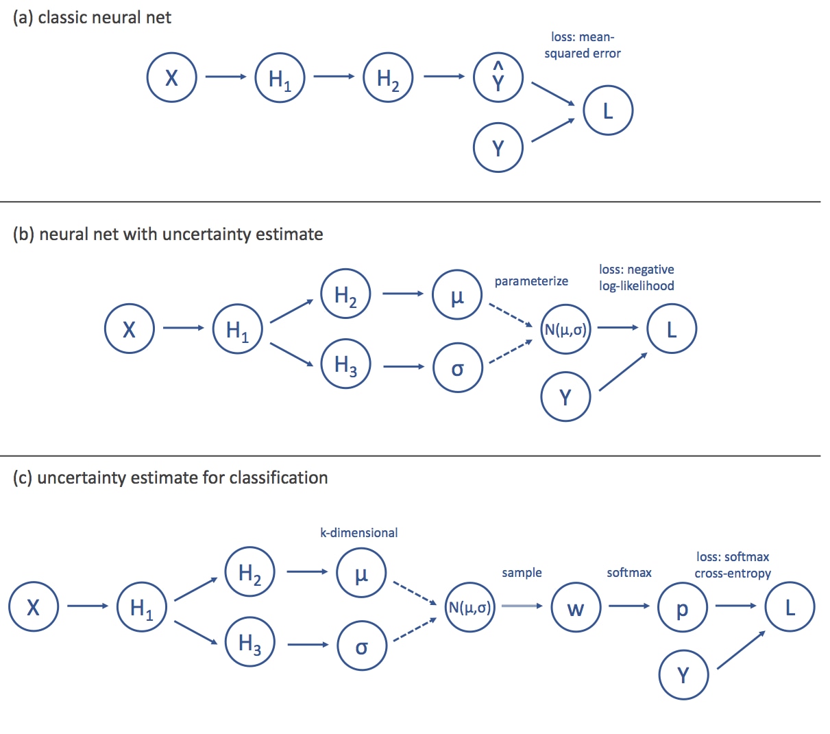
Figure 2 : (a) A high-level depiction of the computational graph for a standard neural network. The input (X) is transformed through multiple hidden layers (Hk), and the final layer produces an estimate (Y) of the target (Y). The loss (L), is then computed as the mean-squared error between Y and Y. (b) To model aleatoric uncertainty, we split the neural network into two streams, the first of which produces an estimate of a mean () while the second produces an estimate of a standard deviation (). Assuming that these parameterize a Gaussian distribution (N(,)), we can then define the loss as the negative log likelihood of the target under this distribution. © For a classification problem with k classes, the standard approach is to have the network output k weights (w) that represent the evidence for each class. These weights are then passed through a softmax function to produce probabilities for each class (p) and the loss is the cross-entropy between the probability vector and the one-hot target. We can model aleatoric uncertainty in this setting by having our network produce the parameters for a k-dimensional Guassian distribution over the evidence weights (instead of the outputs). We then minimize the average cross-entropy loss over samples from this distribution.
Modeling uncertainty in deep neural networks
Modeling aleatoric uncertainty comes down to having a model predict a distribution over outputs rather than a point estimate. One way to do this is to have the model predict the parameters of a distribution as a function of the input. From this perspective, traditional neural networks (Figure 2a) actually already capture a form of aleatoric uncertainty. Consider the standard mean-squared loss that most neural networks minimize:

Where W are the network weights, fW() is the function defined by the network, (xk,yk) is the k-th training example, and N is the number of training examples. Multiplication of addition by a factor that is independent of the weights will not change the optimization objective defined by the loss, so this loss if equivalent to

Where is an arbitrary constant. This is significant, as this is equivalent to the log-likelihood of the data under a Gaussian distribution with mean fW(xk) and standard deviation , i.e.

From this perspective, a standard neural network can already be interpreted as a probabilistic model where each input is mapped to a distribution over possible outputs. However, the fixed standard deviation means that it only handles the relatively uninteresting homoscedastic case where the aleatoric uncertainty remains constant; in many real world applications, it is unreasonable to assume that uncertainty will not vary as a function of input.
To handle the heteroscedastic case, we can modify the architecture of our neural net (Figure 2b) such that we split the layers into two “streams” at some point along the feed-forward chain, producing two outputs: fW(xk) and gW(xk). We can then interpret one as the mean, (xk), and the other as the standard deviation,(xk), which is the quantification of aleatoric uncertainty that we have been looking for. Finally, we define our loss function as the log-likelihood as before:

In the first term of the above equation, we see that inputs with high values of predicted uncertainty actually have the accuracy of the prediction count less toward the loss. This has the nice property of allowing the model to attenuate the impact of less likely outcomes on model training. On the other hand, the second term can be interpreted as a penalty against overuse of this tactic to minimize the loss. In this way, this straight-forward probabilistic approach to modeling aleatoric uncertainty automatically regularizes our model against over-fitting. This regularization often leads to increases in performance on-par with what you would normally only get with extensive (and expensive!) hyperparameter tuning (Figure 1c-f).
In general, this technique can be extended to other distributions as well. We simply split the neural network output into as many components as there are parameters in the distribution we want to use to model the aleatoric uncertainty and then use maximum likelihood as the objective function. The approach can also be extended to classification with a little more work (Figure 2c).
In the traditional approach, the final unscaled activations (one per class) are passed through a softmax function to scale them so they sum to 1. The loss is then computed as the probability of the correct class (also known as the softmax cross entropy loss). Unfortunately, the softmax outputs from a network trained in this way are not true probabilities over the classes in the sense that we want for aleatoric uncertainty. Furthermore, the prediction targets are now labels corresponding to classes, and there is no easy way to parameterize a distribution over such objects. A work-around is to model a k-dimensional Gaussian distribution (where k is the number of classes) over the unscaled activations. The loss function can then be defined as the standard softmax cross entropy.
MNIST example
Finally, we have reached the MNIST example. The internet abounds with tutorials for training convolutional neural networks using the MNIST dataset. It has become such a reference point that even Tensorflow ships with the MNIST data. The model that most beginners learn when working with MNIST is the two-layer convolutional neural network, with max pooling and dropout. We won’t go into much detail on the specifics of filters and kernel sizes (which are widely covered on the web). Suffice it to say that the standard model passes the outputs of the second max pooling layer into a dense layer (applying dropout along the way). There is a final dense layer where the network is squashed down to the number of categories (10 digits) before being passed into a softmax categorical cross-entropy loss function. We then adapt the network to model aleatoric uncertainty with approximately seven additional lines of code, as can be seen below.

Figure 3: Sample code for modifying traditional MNIST convolutional neural network to predict aleatoric uncertainty.
This takes the output of the second dense layer and uses it to predict two things: the locs (means) and scales (standard deviations) of 10 normal distributions (one for each digit). Then we sample 1,000 times from those distributions;for each sample compute the softmax categorical cross entropy (same as before, except now for every input “x,” we tile the true label 1,000 times). The full architecture for this model can be seen in Figure 4. In the past you would have to explicitly tell Tensorflow to skip the normal distributions in the backwards pass, but recent incorporations of Edward into Tensorflow have made this a native functionality.

Figure 4: Network architecture of Bayesian reparameterized MNIST CNN
Simply using this model and no hyperparameter tuning, we were able to achieve an accuracy of 99.33%. The original MNIST model we reparameterized achieved a performance of around 97%. This result puts us in the top 35 for models trained on this data. Many of the other models in the top 35 either required either very deep neural networks to achieve their results or a significant amount of hand-tuning and crafting to get their performance. It is a fascinating by-product that allows a model to learn to predict a label and, it is further interesting to see that uncertainties over all possible labels had such a profound effect on the model’s performance.

Benchmark results compiled here.
Perhaps more interesting is what you can do once you have learned this posterior distribution. As you can see in the examples, after having trained the neural network, you can pass in a new observation and recover the predicted means and standard deviations for each class. These are values before they have been squashed by the softmax. In the first case (digit 8), the spike all the way to the right indicates that the model is fairly confident that it is an 8. However, for the three in the next image you can see that the spread between the mean of the distribution at 3 and the distribution at 8 is not that large. Furthermore, the standard deviations for both these classes indicates aleatoric uncertainty when the model tries to distinguish between these two classes.

Figure 5: Distributions over softmax inputs for two example digits (eight and three). Each row contains the predicted gaussian distribution over that digit. Values further to the right indicate stronger evidence for that digit. Units are not included as only relative distances matter prior to the softmax transformation.
We can see this type of behavior more clearly in the two examples below by zooming in on the model’s predicted distributions for the top three most likely classes. In the case of the 9, this model predicts an 8, but the distribution of the 8 overlaps with that of the 9. The model’s prediction has high uncertainty. This is even more extreme for the 6.

Figure 6: Distributions over softmax inputs for two example digits (nine and six). Only the relevant subset of softmax inputs are shown here to highlight overlap.
Conclusion
As you can see, this methodology allows us to marry the power and flexibility of neural network models combined with the uncertainty quantification of a probabilistic approach. In a business context, especially where risk mitigation and algorithmic uncertainty become critical, this marriage impacts both the ability to make business decisions based off of models in addition to improving the underlying models’ performance. At Capital One, we are actively exploring the applications of these methodologies to challenging industry problems, and we look forward to sharing more updates and insights!
More reading on the topic
- Dropout as a Bayesian Approximation: Insights and Applications
- Dropout as a Bayesian Approximation: Representing Model Uncertainty in Deep Learning
- BAYESIAN CONVOLUTIONAL NEURAL NETWORKS WITH BERNOULLI APPROXIMATE VARIATIONAL INFERENCE
- On Modern Deep Learning and Variational Inference
- What Uncertainties Do We Need in Bayesian Deep Learning for Computer Vision?
- Concrete Dropout
- Vprop: Variational Inference using RMSprop
- Loss-Calibrated Approximate Inference in Bayesian Neural Networks
- Dropout Inference in Bayesian Neural Networks with Alpha-divergences
- A Theoretically Grounded Application of Dropout in Recurrent Neural Networks
- Understanding Measures of Uncertainty for Adversarial Example Detection


