Machine learning for temporal data in finance
How machine learning methods are evolving to address the complex temporal and sequential elements of consumer financial data.

Time series modeling has always been a core element of finance as investment in the financial industry is largely based on some understanding of future economic and market conditions given current and historical knowledge. Forecasting commodity and stock prices or macroeconomic indicators might come to mind as traditional applications of time series models.
The advancement of technology and the resulting digitization of the industry has fundamentally changed the scope of time series modeling necessary and possible in the financial services industry. This transformation has brought about new streams of data such as detailed debt/credit transaction data, digital credit reports, multichannel payments, check images, and customer clickstream data. While progress in machine learning has accelerated the development of models to leverage this data, there remain gaps between methods designed for static data and methods that can capture the complex temporal and sequential aspects of new data streams.
Capital One researchers Jason Wittenbach, Brian d’Alessandro, and Bayan Bruss comment on the new challenges we face in the financial industry and areas of opportunity for new research in their KDD 2020 Machine Learning in Finance Workshop paper Machine Learning for Temporal Data in Finance: Challenges and Opportunities. In this blog, I provide an overview of their observations and summarize current and past research on the topic of time series.
Broadening the Scope of Time Series Modeling
Commonly, time series are modeled and thought of in finance in the most restricted form. These are uniform time series: a sequence of evenly spaced data points in an explicit order with associated timestamps. There is substantial research into models that address this specific type of data. However, it only applies to a very limited set of problems.
Many financial institutions have numerous temporal data types that lie outside this narrow definition. These are broadly referred to as non-uniform time series. You can probably guess that these allow for data points at irregular intervals. This certainly doesn’t make the modeling any easier. Different theories about how non-uniform time series are generated lead to two sub-classes: irregularly sampled time series and temporal point processes.
Irregularly Sampled Time Series
Irregularly sampled time series can occur in two ways. The first is when we have some continuous time series and we take measurements at irregular intervals. Take for example blood pressure. Blood pressure is continuous, since at any time we want to take a measurement a person’s blood pressure exists and can be measured. The second form is a discrete process that may happen uniformly, but some of the observations are missing. Taking blood pressure measurements daily could also be framed as a uniform discrete process. Missing observations may occur due to doctors’ mistakes, unforeseen medical events, or confidence in a patient’s health. Distinct causes of missing values often lead to “informative missingness”—missing values that provide pertinent information about classification labels such as patient outcomes (Che 2018).

(Wittenbach, d’Alessandro, Bruss 2020)
Temporal Point Processes
Temporal point processes are discrete events where the time in-between events is determined by a probability distribution. A customer making a credit card transaction is a point process. The time until that customer uses their credit card is unknown and random, at least to the observer. Two common point processes are poisson and hawkes processes. They both rely on the concept of intensity or rates where a high intensity results in an increased density of events in a time period. Poisson processes generally describe events where the time to the next event is independent of the the past, while hawkes processes model situations where the time since recent events determines the likelihood of future events.
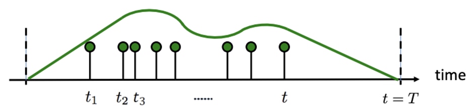
Inhomogeneous Poisson Process (Rodriguez 2018: http://learning.mpi-sws.org/tpp-icml18/seminar-icml18-part1.pdf)

Self-exciting/Hawkes Process (Rodriguez 2018: http://learning.mpi-sws.org/tpp-icml18/seminar-icml18-part1.pdf)
Multivariate and Multimodal Extensions
Non-uniform time series can be expanded even further. So far we have only referenced univariate time series that take on a single value at any time. Financial institutions record so much information about particular events, which means that each event will likely have multiple features associated with it. Financial services companies don’t just record that a credit card transaction occurred, they also store information about the amount, the store, and the location. How should these features be modeled together? For example, how does the sequence of locations and spending amounts in the past relate to the probability of a transaction being fraudulent? At the same time, parallel data streams such as debit card transactions and cash withdrawals/deposits introduces another hierarchy of factors to consider.
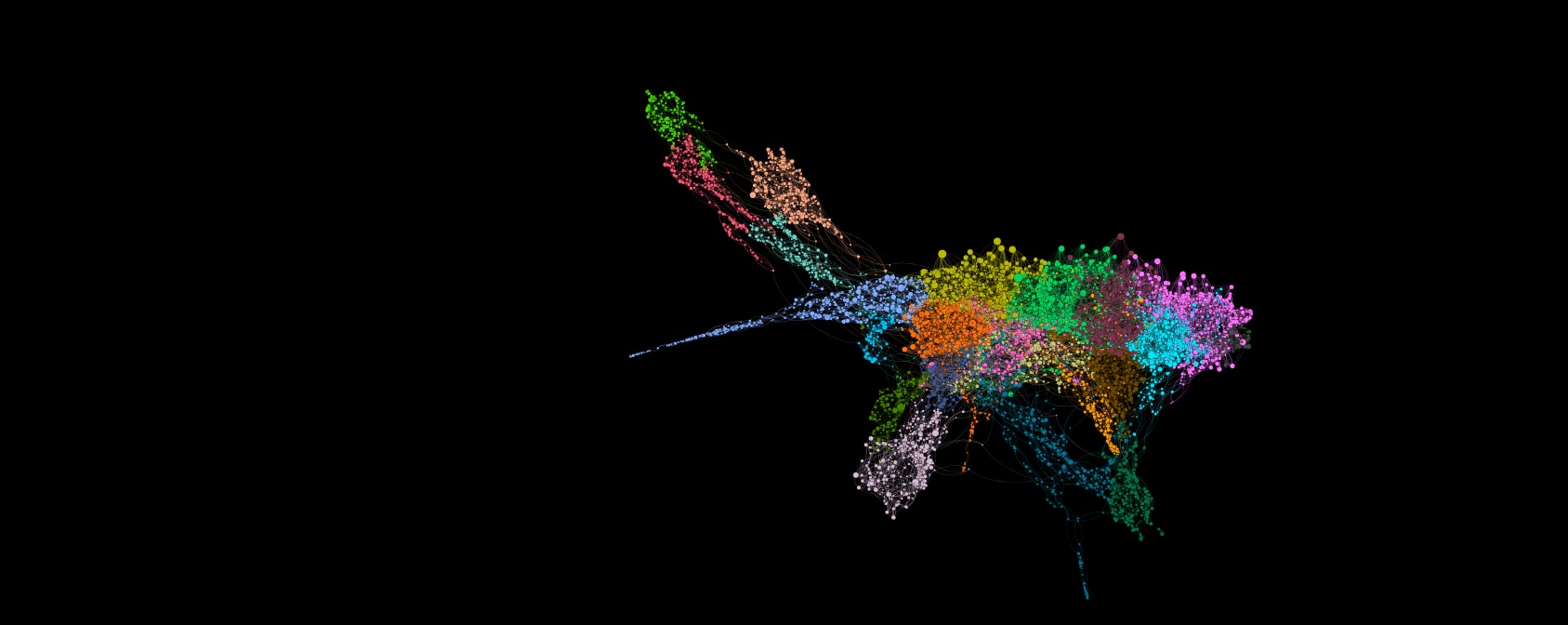
The last layer of complexity comes in the form of different modalities. Common modalities are images, text, graphs, and tabular data. Though the bulk of data in financial services is tabular, other modalities are becoming more common now: sequences of check images from mobile deposits, a customer regularly visiting and traversing the graph of the website, or text from customer service chats online. Modern machine learning has enabled effective representations of these modalities, but new challenges arise when we try to understand their temporal interactions.
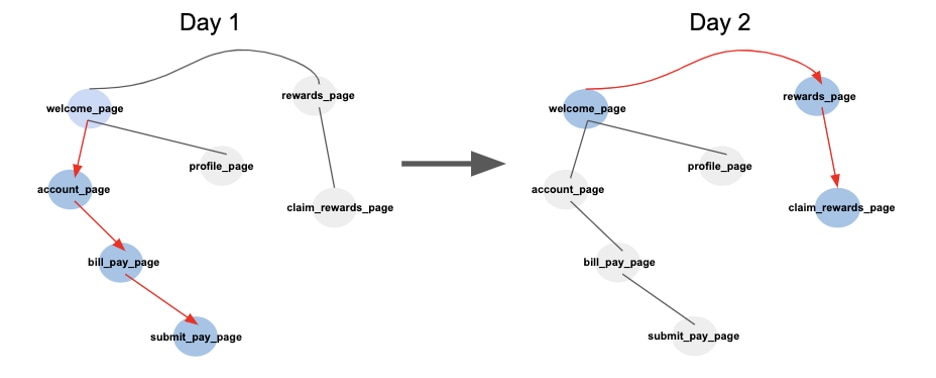
A sequence of website graph traversals (Samuel Sharpe 2020)
Progress in Recent Machine Learning Research
All hope is not lost! Uniform time series have the benefit of decades of research which has focused on statistical autoregressive approaches or methods that decompose into level, trend, and seasonality. Recently, while many different deep recurrent neural networks (RNN) have surfaced, the traditional methods have proven to still be robust and competitive. Only recently have RNN based methods surpassed performance on uniform time series forecasting tasks; it took an approach that mirrored the traditional decomposition model to apply deep learning effectively (Oreshkin 2019).
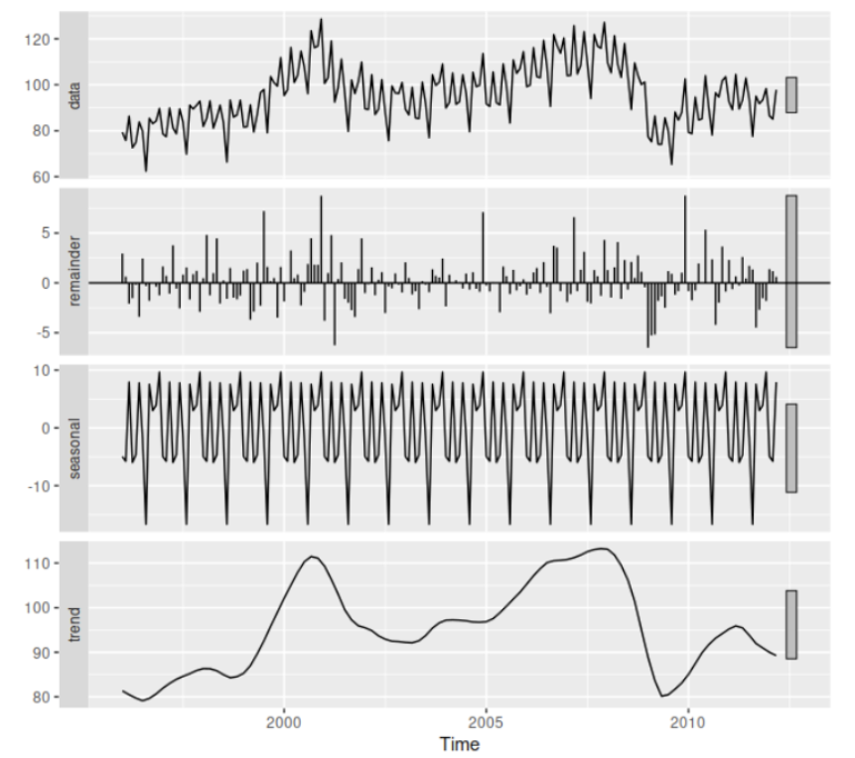
Time series decomposition (Hyndman 2014: https://otexts.com/fpp2/components.html)
Deep learning approaches for non-uniform time series have evolved quickly in the past few years. A common approach to modeling irregular time series is forcing it to be uniform: break it into equally sized bins of time so that only one event occurs at most once in each time period. However, this approach often causes more problems than it solves. How do we fill in the positions with missing data? What if there are few events, but they sometimes occur close together? We would need very small bin sizes and would be unnecessarily blowing up the size of the data. Is the presence of observations or the timing of events important to the task at hand? Researchers have attempted to address these issues by augmenting the data with missing indicators, times between observations, or even incorporating time decay into the architecture of the RNN.
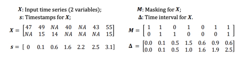
Example masks and time delta features (Che 2018: https://www.nature.com/articles/s41598-018-24271-9.pdf)
To avoid some of the hurdles that these discrete approaches face, research has turned to models designed to directly model the data in its irregular form. Neural networks can be used to parameterize traditional point processes or ordinary differential equations (ODE). Temporal point processes are defined by an underlying intensity, so we can utilize neural networks to model the factors that contribute to this rate at which events occur. A drawback of common point processes is their restriction to a fixed functional form—similar to any probability distribution.
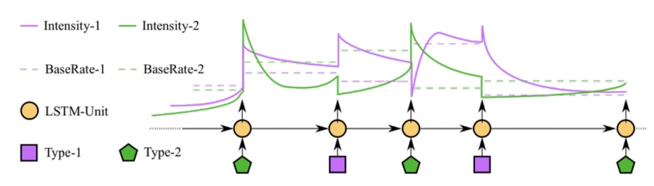
Depiction of a neural hawkes process where “excitement” is modeled with an LSTM cell (Mei 2017: https://www.cs.jhu.edu/~jason/papers/mei+eisner.arxiv17.pdf)
ODEs relate functions to their derivatives or rates of change. The ability to relate complex functions parameterized by neural networks to their rate of change over time allows us to evolve these functions over time without a fixed form or any observation. Neural ODEs have recently augmented RNNs, defining the change in hidden states between observations. Neural augmentation of these methods provide flexible continuous time models of time series, and are thus more realistic for raw data collected by financial services companies.
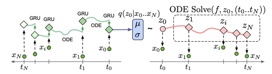
Latent ODE Model with ODE-RNN Encoder (Rubanova 2019: https://arxiv.org/abs/1907.03907)
Progress in continuous time deep learning is accelerating, but hasn’t yet been adopted in multi-modal research. The majority of work on multi-modal fusion has benefited from RNNs, attention mechanisms, and representation learning, and is applied to mostly time agnostic general sequence data. Researchers have developed multi-model fusion models that caption images, align words with speech, recognize emotion with audio and visual cues, match text to localized objects in images, and even align movies and books. Additional work is needed to extend these techniques to continuous and irregular time series data.
Future Challenges and Opportunities
Research into non-uniform time series has provided a path forward for grappling with the irregular temporal aspects of event data streams. Experimentation is the first step for companies in the financial services industry. How can we apply these new methods to our data? Does it drastically improve our understanding of customers? Are there trade-offs with the complexity of new methods such as computation or explainability?
Additional challenges still exist for future work attempting to capture the full dynamics of heterogeneous data. What does current research lack that we need to see the full picture? Will it model multivariate data effectively? Will it combine different data streams thoughtfully? How can it incorporate alternative modalities?
Despite the remaining challenges presented by all these questions, we see significant promise in the study and application of methods to model temporal data in financial services.
Additional Resources
Blogs and Presentations
Forecasting: Principles and Practice
Learning with Temporal Point Processes ICML 2018 Tutorial
Tutorial on Multimodal Machine Learning
Papers
Recurrent Neural Networks for Multivariate Time Series with Missing Values
The neural hawkes process: a neurally self-modulating multivariate point process
References
Oreshkin, Boris N., et al. "N-BEATS: Neural basis expansion analysis for interpretable time series forecasting." arXiv preprint arXiv:1905.10437 (2019).
Che, Z., Purushotham, S., Cho, K. et al. Recurrent Neural Networks for Multivariate Time Series with Missing Values. Sci Rep 8, 6085 (2018). https://doi.org/10.1038/s41598-018-24271-9
Mei, Hongyuan, and Jason M. Eisner. "The neural hawkes process: A neurally self-modulating multivariate point process." Advances in Neural Information Processing Systems. 2017.
R.J. Hyndman and G. Athanasopoulos. 2014. Forecasting: principles and practice . OTexts. https://books.google.com/books?id=gDuRBAAAQBAJ
Rodriguez, M. Gomez, and Isabel Valera. "Learning with temporal point processes." Tutorial at ICML (2018).
Rubanova, Yulia, Ricky TQ Chen, and David Duvenaud. "Latent odes for irregularly-sampled time series." arXiv preprint arXiv:1907.03907 (2019).
Wittenbach, Jason, Brian d’Alessandro, and Bayan Bruss. “Machine Learning for Time Series in Finance: Challenges and Opportunities”. KDD Machine Learning in Finance Workshop (2020).