Learning Embeddings of Financial Graphs
By Bayan Bruss, Lead Software Engineer, Capital One and Keegan Hines, Director of Software Engineering, Capital One
“You are the average of the five people you spend the most time with.” This quote from Jim Rohn emphasizes that we can deduce a great deal about someone simply by knowing their connections. The importance of connections is what drives the study of graphs (aka networks), a field of mathematics that stretches back to the 1700s, and in recent years has become an important topic in machine learning.
For a financial institution, we deal in graphs every day: a credit card transaction is a connection between a merchant and an account holder, a mortgage is a connection between a lender and a homeowner, a wire transfer is a connection between two financial accounts. Indeed, the study of graphs lies at the heart of better understanding our customers and what they need. However, all such graphs are extremely challenging to work with in typical machine learning applications. This is because they are typically very large, with millions (or hundreds of millions) of nodes and billions of edges. At the same time, they are typically very sparse, with each node interacting with only a tiny fraction of the other nodes.
The last few years have seen exciting progress in applying Deep Learning to graphs to solve these problems. However, these techniques have yet to be evaluated in the context of financial services. Graphs hold the promise to help us understand our customers by shedding light on who they connect with, but at the same time, the vastness of this data makes it challenging to bring this perspective into typical business problems. In this blog post, we’ll describe how we’ve overcome these challenges using graph embeddings in order to gain a data-driven understanding of our customers and their economic life. For a more detailed technical description, we encourage readers to look at our recently posted paper which we will be presenting at ICMLA 2019.
Overview of Graph Embeddings
One of the greatest recent advances in Natural Language Processing has been the success of word embeddings. Natural language suffers from many of the problems we just noted about graphs: a language tends to contain millions of unique words and most words appear very rarely alongside any other particular word. The high-dimensionality and sparsity of language makes it challenging to process documents in a way that is useful for common machine learning algorithms. To address this problem, word embedding models seek to learn a low-dimensional vector for each word such that the relative locations of word vector will tend to capture important semantic properties of how words are used in common language. If successful, the learned word embeddings might result in nearby word vector for semantically similar words (synonyms). Further, logical relationships between words and concepts might also get represented. The figure below shows a simplified example of what some word vectors might look like. In the middle figure, note that semantically similar words (such as walking and walked) might appear close to each other. Additionally, these techniques were met with great excitement as the embeddings seem to allow us to do analogical reasoning using only vector arithmetic on these word vectors. The verb-tense change of “walking to walked” corresponds to the same direction in the embedding space as the verb-tense change of “swimming to swam”. The left of Figure 1 shows the now-classic analogy “King is to Man as Queen is to Woman”, visualized as vector operations in this space. These word embedding techniques proved to be very successful at capturing the semantic meanings of words in completely data-driven way.
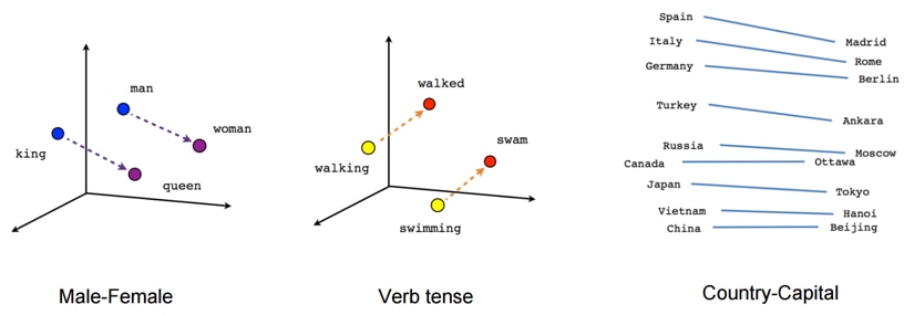
Figure 1: Simplified example of word embeddings. Source: TensorFlow, https://www.tensorflow.org/tutorials/representation/word2vec
Taking inspiration from the success in NLP, researchers who study graph algorithms quickly devised adaptations that could work in this domain. Here, the goal would be to learn an embedding for each of a graph’s nodes such that the geometry of the embedding space would roughly capture the relationships of the graph. Sticking close to the NLP workflow, algorithms such as node2vec and DeepWalk posit that by simply generating random walks on graphs, we can use these sequences of nodes as input “sentences” into a model very similar to word2vec. Later efforts sought to tackle additional complexity such as how to include node attributes and how to handle multiple kinds of nodes or multiple kinds of edges.
Our Methodology
We can consider credit card transactions as edges in a bipartite graph with two distinct kinds of nodes (accounts and merchants). Each transaction adds weight to an edge that joins an account to a merchant. This graph is said to be bipartite because these edges only ever occur between account nodes and merchant nodes. For example, there would never be an account-to-account credit card transaction. Thus, our goal is to learn an embedding of this bipartite graph so that we have a dense vector representation for each account and for each merchant. If things work out well, then accounts will be embedded near each other if and only if they tend to shop at the same kinds of merchants. And merchants will be embedded near each other if and only if they tend to receive customers who have similar shopping habits.
For the results we describe below, we’ll focus exclusively on the merchant vectors, as they are familiar entities that we can reason about and check against our intuition. For this analysis, we’ve collapsed the “raw merchant” from the card transaction into its brand name. As an example, every Starbucks franchise would show up uniquely in the transaction logs according to their store number and physical location. However, we’ve chosen to combine all these into a single Starbucks entity for much of this analysis (see the accompanying paper for details on the much larger raw merchant graph).
To tackle the problem of having to embed a bipartite graph, we’ve chosen to induce two homogeneous graphs by projecting the bipartite graph. As shown in the figure below, two merchants in the bipartite graph might share the same account who shopped at both of them (such as Merchant A and Merchant B sharing Account A). In the projection graph, we would get a homogenous graph of only merchant nodes, and there is an edge between Merchant A and Merchant B to denote that they shared a customer in the original graph. Implicitly, that edge is weighted the more frequently customers shop at both merchants. Conversely, we can construct an account project graph by linking accounts who shop at the same merchant. It is important to consider transactions that occur close in time, otherwise the entirety of the graphs would be fully connected. For our purposes, we found that it is effective to consider two accounts as connected if they shop at the same merchant within the same day. And for merchants, a might smaller time window is needed, since each merchant sees such a higher volume of transactions.
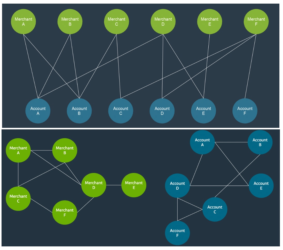
Figure 2: Simulated graphs derived from credit card transactions. (Top) Transactions induce a bipartite graph between Accounts and Merchants, with each edge representing a transaction. (Bottom) Projections of bipartite graphs into two homogenous graphs.
With these homogeneous graphs, we can proceed in a fashion very similar to the algorithms previously described. By taking short random walks on this graph, we can generate sequences of entities that can be trained using a word2vec-like model.
Results
Once we’ve trained our model from card transactions, one would hope that the learned embeddings tend to capture intuitive similarities about these entities. In much the same way that nearby word vectors tend to be synonymous words, it is interesting to examine if nearby merchant vectors are similar in any meaningful way. In order to ask this question, we can fetch the embeddings for common household brand merchant and search the embedding space for their nearest neighbors. The table below shows some encouraging results.

Fig 3: Merchant nearest neighbors derived from the brand-level merchant graph. For each query merchant vector (in bold), the top three nearest neighbor merchant vectors are shown.
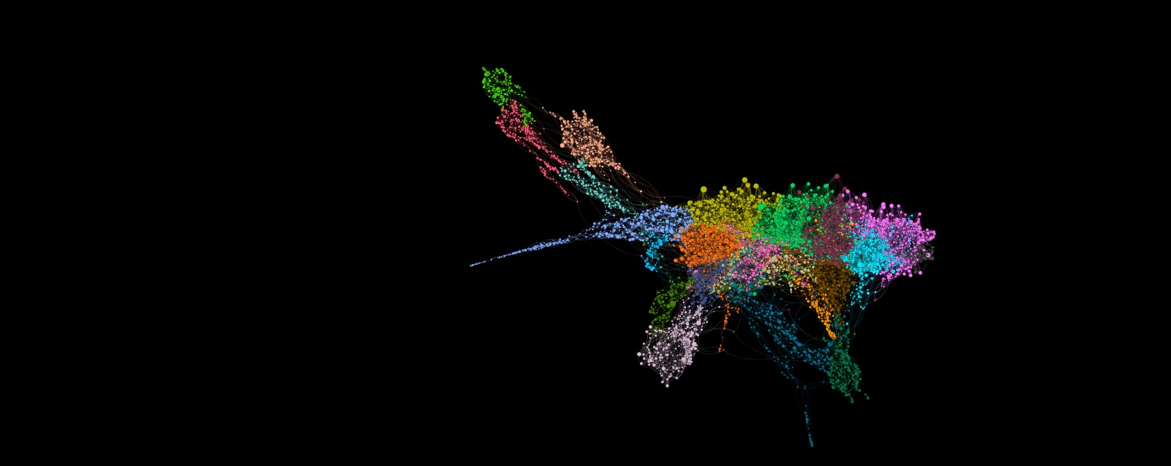
For each query merchant (in bold), we see the top-3 nearest neighbor merchant vectors. We see that the nearest neighbors of the KFC merchant are not only other restaurants, but other fast food brands. This pattern holds true over several industries including fashion, dining, transportation, and furniture. The figure below shows a two-dimensional visualization of the mechant embedding space. This trend of separability-by-industry continues across the whole landscape. Zooming in on this figure reveals distinct clusters of merchants according to their category such as sporting goods, fast food, travel, retail, and so on. Indeed, this approach of embedding the transaction graph was able to capture the similarity of these entities in a way that is consistent with our intuition about these brands.

Example clusters found in a two dimensional t-SNE projection of brand-level embeddings.
A final set of questions we can ask with these brand-level merchant embeddings is whether relationships between merchants can be consistently observed within and between industries. In much the same way that analogical reasoning tasks can be accomplished with word vectors (see Figure 1), it might be feasible to identify compelling relationships between merchant vectors.
One way to construct analogies for merchants is to devise relations between merchants within one category and determine if the same relationship holds across categories. As a concrete example, we can recognize that within a particular industry, there will exist several offerings that are not direct competitors but instead operate at different price points. For example, within automobiles, the typical Porsche price point is well above that of Honda, though they offer the same basic good. If there is a direction in the embedding space that encodes price point (or quality or luxury) then this component should contribute to all merchants across all industries. In this way, the embeddings can elucidate analogies such as "Porsche is to Honda as blank is to Old Navy.'
For our purposes, we assumed that such a direction, if it existed, was likely a dominant source of variation between the embeddings and that this direction is likely captured by one or a few principal components of variation. With this in mind, we identified several pairs of merchants which exist in the same category yet span a range of price points. These included: {Gap and Old Navy}, {Nordstrom and Nordstrom Rack}, {Ritz-Carlton and Fairfield Inn}, and so on. These pairs were chosen because they represent nearly identical offerings within a category, but at a high and low price point. In Figure 5, we visualize these paired merchant vectors as projected into a convenient subspace spanned by two principal components. Interestingly, the relationship (slope) between the low-end and high-end offering is nearly parallel for all of these pairs. There indeed exists a direction in the embedding space which encodes price point and this direction is consistent across these disparate industries.

Fig 5: Merchant embeddings tend to encode typical price point of goods. Merchants from multiple industries visualized in the subspace spanned by the fourth and fifth principal components. Pairs of merchants are joined by dotted lines, with each pair containing a high-end merchant and a more affordable counterpart. Across disparate industries, the relationship between high-end offerings and affordable offerings is embedded in a consistent direction of this space.
Apart from the qualitative analysis presented here, the accompanying paper reports quantifications of the efficacy of these embeddings over various regimes and for common graph-analytic tasks.
Conclusions and Future Directions
In this post, we’ve described how we can apply the idea of embeddings to important problems in financial services. By analyzing graphs of credit card transactions, we can use representation learning to understand how entities are similar based on how they interact. Excitingly, this approach can yield intuitive results that capture our “semantic” understanding of these financial entities. The techniques described here just scratch the surface of what is possible. It will be very exciting to extend to more sophisticated techniques that capture more than just graph topology to include ancillary information that is known about transactions, accounts, and merchants. Even more compelling is the possibility of using these representations for downstream business needs.
Learn more in our upcoming ICMLA paper.