Understanding ARIMA models for machine learning

In a world driven by data, the ability to forecast future trends is essential across industries — from financial markets to supply chain planning. One method that plays a central role in time series forecasting is the ARIMA model, short for Autoregressive Integrated Moving Average. Known for its statistical rigor and versatility, ARIMA helps uncover patterns in historical data to inform short-term predictions. In this article, we’ll take a closer look at how ARIMA models work, when to use them and what their advantages and limitations mean for machine learning and beyond.

The autoregressive integrated moving verage (ARIMA) model is applied across various industries. It is widely used in demand forecasting, such as in determining future demand in food manufacturing. That is because the forecasting model provides managers with reliable guidelines in making decisions related to supply chains. ARIMA models can also be used to predict the future price of your stocks based on past prices. Although ARIMA models can forecast general trends in financial markets, they are not reliable for predicting abrupt, speculative events—such as the unexpected spike in GameStop (GME) stock.

That’s because ARIMA models are a general class of models used for forecasting time series data. ARIMA models are generally denoted as ARIMA (p,d,q), where p is the order of the autoregressive models, d is the degree of differencing and q is the order of the moving-average models. ARIMA models use differencing to convert a nonstationary time series into a stationary one and then predict future values from historical data. These models use “auto” correlations and moving averages over residual errors in the data to forecast future values.

• Only requires the prior data of a time series to generalize the forecast.

• Performs well on short-term forecasts.

• Models nonstationary time series.

• Difficult to predict turning points.

• Quite a bit of subjectivity involved in determining (p,d,q) order of the model.

• Computationally expensive.

• Poorer performance for long-term forecasts.

• Cannot be used for seasonal time series.

• Less explainable than exponential smoothing.

Let’s say you want to predict a company’s stock price with an ARIMA model. First, you will have to download the company’s publicly available stock price over the last few — let’s say 10 — years. Once you have this data, you are now ready to train the ARIMA model. Based on trends in the data, you will choose the order of differencing (d) required for this model. Next, based on autocorrelations and partial autocorrelations, you can determine the order of regression (p) and order of moving average (q). An adequate model can be selected using Akaike Information Criterion (AIC), Bayesian Information Criterion (BIC), maximum likelihood and standard error as performance metrics.

As stated earlier, ARIMA(p,d,q) is one of the most popular econometrics models used to predict time series data such as stock prices, demand forecasting and even the spread of infectious diseases. An ARIMA model is basically an ARMA model fitted on d-th order differenced time series such that the final differenced time series is stationary. 

A stationary time series is one whose statistical properties, such as mean, variance and autocorrelation, are all constant over time. A series is relatively easy to predict — you simply predict that its statistical properties will be the same in the future as they have been in the past!

To understand how an ARIMA model functions, there are three terms within the name that you will need to better understand:

• AutoRegressive: AR(p) is a regression model with lagged values of y, until p-th time in the past, as predictors. In the following formula, p is the number of lagged observations in the model, ε is white noise at time t, c is a constant and φs are parameters:

• Integrated I(d): The difference is taken d times until the original series becomes stationary. A stationary time series is one whose properties do not depend on the time at which the series is observed.

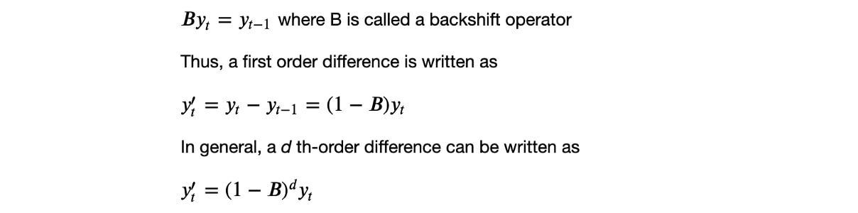
Let’s look at two graphs from Forecasting: Principles and Practice (2nd ed) by Rob J Hyndman and George Athanasopoulos. Graph (a) on the left is Google’s stock price for 200 consecutive days. This is a nonstationary time series. Graph (b) on the right side is the daily change in the Google stock price for 200 consecutive days. Image (b) is stationary because its value does not depend on the time of observation. In this example, the order of differencing would be one, as the first-order differenced series is stationary.

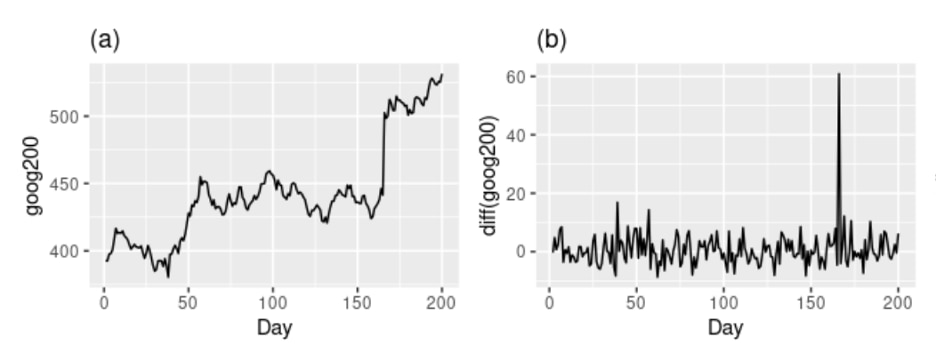
Graphs taken from Forecasting: Principles and Practice (2nd ed) by Rob J Hyndman and George Athanasopoulos (https://otexts.com/fpp2/arima.html)

• Moving average MA(q): A moving average model uses a regression-like model on past forecast errors. Here, ε is white noise at time t, c is a constant and θs are parameters:

Combining the above three types of models gives the resulting ARIMA(p,d,q) model:

The ARIMA methodology is a statistical method for analyzing and building a forecasting model that best represents a time series by modeling the correlations in the data. Owing to purely statistical approaches, ARIMA models only need the historical data of a time series to generalize the forecast and manage to increase prediction accuracy while keeping the model parsimonious.

Despite being parsimonious, there are multiple potential disadvantages to using ARIMA models. Most important of them stems from the subjectivity involved in identifying p and q parameters. Although autocorrelation and partial autocorrelations are used, the choice of p and q depends on the skill and experience of the model developer. Additionally, compared to simple exponential smoothing and the Holt-Winters method, ARIMA models are more complex and thus have lower explanatory power.

Lastly, similar to all forecasting methods, by being backward-looking, ARIMA models are not good at long-term forecasts and are poor at predicting turning points. They can also be computationally expensive.

Thus, ARIMA models can be easily and accurately used for short-term forecasting using only time series data, but identifying the optimal set of model parameters for each use case may require experience and experimentation.

Thus, ARIMA models can be easily and accurately used for short-term forecasting using only time series data, but it can take some experience and experimentation to find an optimal set of parameters for each use case.

For more resources, check out some projects using the ARIMA method: 

• How to Create an ARIMA Model for Time Series Forecasting in Python

• ARIMA Model – Complete Guide to Time Series Forecasting in Python

• Time Series Analysis Using ARIMA Model In R

New to tech at Capital One? We touch every aspect of the research life cycle, from collaborating with Academia to building leading-edge AI products:

• See how our AI research is advancing the state of the art in AI for financial services.

• Learn how we’re delivering value to millions of customers with proprietary AI solutions.

• Explore AI research jobs and join our world-class team in changing banking for good.

- - -

References:

1. Investopedia

2. Forecasting: Principles and Practice (2nd ed) by Rob J Hyndman and George Athanasopoulos

3. https://libres.uncg.edu/ir/uncw/f/zhai2005-2.pdf

4. Predict livestock consumption in Tanzania

5. Demand forecasting

6. Application of the ARIMA model on the COVID-2019 epidemic dataset