Cortex Code CLI: Hands-on review of Snowflake's TPC-DS 10TB

AI coding assistants have a frustrating blind spot: they understand your repository but have limited access to what’s actually in your data platform. If you ask ChatGPT or Copilot for a Snowflake-specific query, you’ll likely spend some time debugging syntax errors and providing the correct context. The problem intensifies when you try to ask the AI questions about the data itself. This all results from the fact that the code lives in one world and the data lives in another.

Cortex Code (CoCo) CLI is Snowflake’s terminal-native AI coding agent built on the Claude Agent SDK and purpose-built for the Snowflake data stack. Ideally, it should be able to leverage key Anthropic features, like multi-step reasoning, plan mode and context compactification, while maintaining a deep integration with Snowflake-specific data structures and technology. 

CoCo CLI became generally available in February 2026, with an expansion to dbt and Apache Airflow announced three weeks later. In this post, I share my review based on a structured test across five distinct areas: Catalog discovery, SQL generation and optimization, Streamlit app building, FinOps cost analysis and dbt model generation.

Everything here was run against SNOWFLAKE_SAMPLE_DATA.TPCDS_SF10TCL, the TPC-DS decision support benchmark at 10TB scale factor that is pre-loaded in every Snowflake account. No dataloading, no Marketplace subscriptions, no additional setup required. If you have a Snowflake account, every prompt in this article is reproducible verbatim.

The dataset models a multi-channel retailer with three fact tables sitting at the center of a 24 table star schema: STORE_SALES at 28.8 billion rows, CATALOG_SALES at 14.4 billion and WEB_SALES at 7.2 billion, for a combined 55.8 billion rows across the schema.

Cortex Code CLI is an agentic shell for Snowflake that bridges the gap between your local development environment and your Snowflake account. Unlike generic coding agents whose context stops at the repository level, Cortex Code is Snowflake-aware. It is grounded in your catalog, permissions, query history, costs and semantic models. It generates SQL and executes it, validates the output and iterates—all within a governed perimeter where your credentials stay local. 

The CLI connects directly to your Snowflake account using existing authentication methods and can execute SQL commands, view tables, validate Cortex Analyst semantic models and manage multiple connections at once. It reads and writes to local repositories making it ideal for managing dbt projects or Streamlit apps. It can also invoke local bash commands and git operations. 

In addition to supporting Snowflake workflows end to end, Cortex Code CLI is now expanding native support to all data systems, starting with dbt and Airflow. Importantly, CoCo is also Snowflake’s first standalone subscription model, with the subscription covering the cost of the LLM inference powering the agent.

Getting started takes one command:

Cortex Code CLI is available across operating systems on Linux, macOS and Windows (WSL and native). Running cortex after installation launches a setup wizard that reuses your existing ~/.snowflake/connections.toml. If you already have the Snowflake CLI configured, you’re connected in under a minute. Your Snowflake user needs the SNOWFLAKE.CORTEX_USER database role, which is granted to all users through PUBLIC by default, but may have been revoked in your organization.

Step 1: Install. Run the curl command above. The script installs the cortex executable in ~/.local/bin by default. Verify the installation with cortex --version.

Step 2: Configure a connection. Running cortex launches the setup wizard. You’ll be prompted to either select an existing connection from connections.toml or create a new one. For this review I was able to reuse an existing Snowflake CLI connection with key-pair authentication. 

Step 3: Verify access. Once connected, type a natural language prompt like “What databases do I have access to?” to confirm the agent can reach your account. If LLM-backed features don’t respond, confirm your user has the CORTEX_USER role. 

Step 4: Set your warehouse. The X-Small warehouse that most accounts default to will time out on full scans of multi-billion row tables. For TPC-DS at SF10TCL, consider a Small or Medium warehouse for the analytical queries. For metadata-only operations (schema introspection, catalog discovery) X-Small is just fine.

The first thing I wanted to answer was simple: Does Cortex Code actually understand what's in my account, or does it just pass my question to a generic SQL generator?

Prompt: “What databases do I have access to? For each one, show me the schemas and a rough count of tables/views.” 

The agent didn’t need to ask for clarification here. It issued two SQL queries autonomously. First a SHOW DATABASES to enumerate accessible databases, then a query against INFORMATION_SCHEMA.TABLES to count objects per schema. It then synthesized the results into a clean summary table. Six databases were returned including SNOWFLAKE_SAMPLE_DATA with its six schemas. 

A general-purpose coding agent given this prompt is likely to generate a SHOW DATABASES call and stop there. CoCo understood that “schemas and rough count” meant a second joined query and produced a table that was actually useful for navigation.

Prompt: “List all the tables in TPCDS_SF10TCL with row counts and column count, sorted by row count descending.” 

Here we got an immediate and complete answer: all 24 tables with actual row counts from INFORMATION_SCHEMA.TABLES.STORE_SALES alone are 28.8 billion rows across 23 columns. The three primary fact tables account for roughly 50 billion rows and the three returns tables add another 5 billion. Total dataset: approximately 55.8 billion rows.

Prompt: “Describe the star schema structure. Identify fact tables, their FK columns and the dimension tables they reference.” 

TPC-DS doesn’t use formal FOREIGN KEY (FK) constraints in Snowflake. The relationships exist conceptually in column naming conventions, not in the DDL. To answer this correctly, the agent had to infer schema structure from column names, not from metadata. 

CoCo issued two queries: 

1. A query to identify primary key candidates in dimension tables (columns ending in _SK).
2. A query to pull all columns from the fact tables to match FK patterns. 

It correctly produced a complete relationship map: 7 fact tables identified, 17 dimension tables catalogued and a detailed FK mapping for each. The CATALOG_SALES mapping alone has 18 FK relationships, including dual customer references pointing to CUSTOMER for both bill-to and ship-to parties.

Prompt: “Compare the column structure of STORE_SALES, CATALOG_SALES and WEB_SALES. Which columns are shared? Which are unique?” 

The agent normalized column names by stripping channel prefixes (SS_, CS_, WS_) before comparing, a meaningful act of semantic reasoning. It then correctly partitioned the columns into four groups:

The agent’s summary captured a business insight inferred from the column structure: “Store sales have simpler customer tracking since the transaction happens in person. Catalog and web sales track separate billing and shipping parties.”

Prompt: “Identify which dimension tables are slowly changing. Show an example of a duplicated key and how versions differ.” 

This was one of the most impressive results. Detecting Type 2 SCDs from raw data requires understanding the concept, identifying candidate tables by looking for date-range columns and validating the pattern with actually duplicated business keys.

The agent ran three queries and correctly identified 5 SCD tables: ITEM, WEB_PAGE, STORE, WEB_SITE and CALL_CENTER. They all followed an exact Type 2 pattern with surrogate key, natural key and date ranges. The agent surfaced concrete examples: 

1. An item reclassified from “Electronics/musical” to “Music/classical” between 1997 and 2000.
2. A store that changed its name and manager while floor space stayed constant.

Prompt: “Write a query that shows total net paid and total quantity by store for calendar year 2001.”

Clean, immediately executable SQL. The agent correctly joined STORE_SALES to DATE_DIM for the year filter and to STORE for the dimension, using the proper surrogate key joins. It also flagged a NULL row in the output (sales records where SS_STORE_SK didn’t join to a valid store), noting it as a data quality observation without being asked. Catalog, discovery, verdict.

Across these prompts, Cortex Code demonstrated three things general-purpose agents consistently fail at:

• Schema inference without constraints: Inferring all FK relationships from column naming conventions
• Semantic normalization: Stripping channel prefixes to compare equivalent columns 
• SCD detection from raw data: Multi-step analytical reasoning, not just prompt-following

Prompt: “Find the top 10 item categories by total net paid across STORE_SALES for Q4. Include item class and average selling price.”

The generated SQL was correct. It ran, but then it timed out against the SF10TCL dataset.

What happened next matters. The agent didn’t retry silently or pretend the query succeeded. It surfaced the failure directly and offered three concrete options: use a smaller scale factor, upsize the warehouse or add date filters. No hallucinated result, no confident fabrication. It told the truth and provided a path forward.

After rerunning against SF1000, it returned results and noted something I would have missed: The average selling price was almost identical across all ten categories ($37.85–$37.88). The agent correctly identified this as an expected property of synthetically generated benchmark data. It knew it wasn’t a data anomaly.

Prompt: “Show each customer’s total spend across all three sales channels in 2002. Rank by total cross-channel spend, top 25.”

This is genuinely one of the harder patterns in TPC-DS. The three fact tables use different column prefixes, carry different FK structures for customer references and need to be joined correctly to a shared CUSTOMER dimension.

Cortex Code produced a clean UNION ALL across all three channels, correctly used CS_BILL_CUSTOMER_SK as the primary customer reference in catalog sales (not CS_SHIP_CUSTOMER_SK) and joined all three to CUSTOMER and DATE_DIM before aggregating.

As you can see in the above table, Store spend dominates for every top customer, typically accounting for +90% of their total. Six of the top 25 customers spent exactly $0 on Web in 2002. The agent surfaced these observations without being asked.

Prompt: “Calculate return rate by item category for STORE_SALES joined to STORE_RETURNS. Flag categories above 10%.”

Cortex Code correctly handled the canonical fact-to-fact join through SS_ITEM_SK and ticket number, producing a 4-table join. No category exceeded 10%: Every category sat at almost exactly 5.15% return rate by quantity, 5.72–5.73% by dollar value. The agent correctly attributed the uniformity to synthetic data characteristics.

Prompt: “The store revenue query is running slowly. Analyze it and suggest clustering keys, pruning improvements, or rewrite strategies.”

The first metadata query failed: STORE_SALES has no clustering key. Rather than silently skipping, the agent pivoted to an execution plan analysis via EXPLAIN and pulled storage metrics from INFORMATION_SCHEMA. It correctly diagnosed: STORE_SALES scans all 8,240 partitions (140 GB) despite filtering for a single year, because the D_YEAR filter lives on DATE_DIM, not on STORE_SALES.

The agent also provided five distinct recommendations with concrete DDL:

• Failure handling is honest and productive. Timeouts were surfaced with concrete alternatives. 
• Failed metadata queries triggered pivots. No fabricated results. 
• Multi-fact joins are correct. Three different column naming conventions, a dual-customer reference and a year filter through a dimension join, all correct on the first attempt. 
• The optimization output is genuinely useful. Five ranked recommendations with actual DDL is the kind of analysis that typically requires a Snowflake specialist.

Before writing a single line of code, CoCo invoked its built-in skill system and read two internal documentation files (~335 lines). It consulted its developing-with-streamlit and connecting streamlit-to-snowflake skills proactively. As a result it generated code that follows Snowflake’s recommended Streamlit connection patterns, rather than generic boilerplate.

The agent autonomously switched from TPCDS_SF10TCL to TPCDS_SF1000 because the larger dataset had caused timeouts in the SQL section. No re-prompting. That’s context persistence doing real work.

Five apps, five first-pass successes

Design decisions worth noting: The return rate scatter plot added bubble sizing to encode quantity sold (a third dimension, unprompted). The multi-channel dashboard chose Altair over st.bar_chart for proper tooltip and stacked encoding support. The customer lookup implemented a two-query, row-selection drill-down pattern requiring coordinated session state management.

• The skill system produces better code. Session memory saves debugging time. The agent makes design decisions rather than just following instructions. 
• Limitation: None of these were deployed as Streamlit-in-Snowflake apps. Deploying to Snowsight still requires a browser handoff at certain steps.

If the SQL and Streamlit tests demonstrate what Cortex Code can build, the FinOps section demonstrates something more unusual: it can look back at what it just did, measure the cost and tell you how to do it more cost-effectively next time.

Prompt: “What are my top 5 warehouses by credit consumption over the past 30 days?”

One warehouse. 427 queries on a single X-Small COMPUTE_WH. Total: 71.71 credits (~$215 at standard pricing). The agent correctly queried WAREHOUSE_METERING_HISTORY (not INFORMATION_SCHEMA, which lacks per-query attribution).

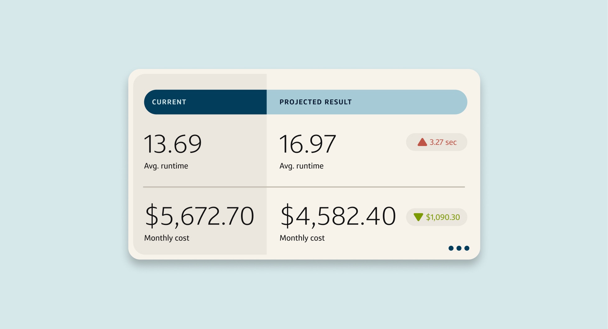
Prompt: “Compare cost of a full STORE_SALES scan on X-Small vs Medium. Recommend the right size for ad-hoc analytics.”

The key finding, correctly derived from actual query data:

Credit consumption is nearly identical across sizes. Snowflake’s per-second billing means a Medium running for 3 minutes costs the same as an X-Small running for 12. For large scans, bigger is not more expensive, it’s just faster. A non-Snowflake-aware agent would likely recommend a smaller warehouse to save money, which would be wrong.

Prompt: “Find the 10 most expensive queries against TPCDS_SF10TCL in the past 7 days.”

What came back was a direct audit of this article’s testing session. The top 3 queries were recognizable from the SQL generation tests: category aggregation (180s, 35.5 GB), Q4 dates CTE (154.7s, 54.9 GB) and store revenue by year (88.9s, 25.5 GB). The agent had effectively closed the loop: Wrote SQL, ran it, then analyzed the cost of running it, in a single session.

Five queries were flagged as full-scan offenders. Three scanned 100% of partitions: Return rate, promotional lift and income band spend all inherently whole-dataset queries by design. The agent correctly identified this and proposed: Clustering keys for date-filtered workloads, explicit date constraint rewrites and a SAMPLE(10) approach for exploratory analysis where directional accuracy is sufficient.

The SAMPLE suggestion is particularly Snowflake-native. It’s a Snowflake-specific clause that many engineers don’t reach for, but which would have produced statistically equivalent conclusions in one-tenth the scan time.

The agent generated a complete per-user attribution report and, unprompted, created a monitoring view:

• It audited itself. The ability to close the write-run-analyze loop in a single session is genuinely novel. 
• The warehouse sizing math is correct and specific. Bigger warehouses cost the same but run faster—the single most useful piece of Snowflake cost guidance for new users. 
• It distinguished signal from noise. Identifying that six full-table scans were on dimension tables and therefore not worth flagging. This determination required the agent to understand both context and table sizes.

The dbt tests were structured as a deliberate escalation: start with a single staging model, build toward a mart, refactor for production, add testing, extend to multi-channel and finally ask for the whole project at once.

Prompt: “Generate stg_store_sales.sql that selects from STORE_SALES, renames columns to snake_caseand casts SS_SOLD_DATE_SK to a proper date.”

Four files written: dbt_project.yml, sources.yml, stg_store_sales.sql and stg_store_sales.yml (61 lines of column docs and tests). The model resolved SS_SOLD_DATE_SK into an actual date at the staging layer. It applied correct dbt architecture without any prompting.

Prompt: “Create mart_store_revenue.sql that joins stg_store_sales to ITEM and STORE dimensions with monthly revenue by category and store.”

The agent read sources.yml before writing. It identified missing source definitions, edited the existing file to add them, then wrote the mart and its YAML documentation. The mart covers the full analytical surface: revenue_month, product and store dimensions, financial metrics and a calculated profit_margin_pct.

Prompt: “Rewrite mart_store_revenue for incremental materialization with a watermark on sold date.”

Two details demonstrate genuine dbt-on-Snowflake expertise: incremental_strategy='merge' generates a MERGE statement (the correct Snowflake strategy) and the one-month lookback ( dateadd('month', -1, max(revenue_month)) ) handles late-arriving data by reprocessing the most recently completed month on every run.

Prompt: “Generate mart_return_rate.sql and add dbt tests for not_null and accepted_values on the channel column.”

103 lines of SQL, 63 lines of YAML. The model added a return_risk_tier calculated column (HIGH/MEDIUM/LOW) and the agent unprompted added an accepted_values test for it. The agent applied the same kind of defensive testing instinct a senior analytics engineer would.

Prompt: “Write mart_customer_ltv.sql calculating LTV across all three channels, using ref() to reference staging models.”

The agent recognized that three staging models didn’t exist yet. Rather than generating a mart referencing nonexistent models, it created all three staging models first, then wrote the 121-line mart with correct ref() chaining. The output schema includes channel-level revenue splits, mix percentages, ltv_tier and channel_engagement labels.

Prompt: “Generate a complete dbt project: staging, intermediate and mart models with schema.yml for every model.”

21 files across three directories. The intermediate layer is the key architectural decision:

Total output: ~494 lines of sources.yml, ~494 lines of schema documentation across three schema.yml files and ~680 lines of SQL across 15 model files. int_sales_unified.sql produces a single UNION ALL view across all three channels, which is exactly the abstraction that prevents the three-way UNION from being rewritten in every mart.

• Project state was maintained. Each prompt built on previously created files. 
• Architecture was applied, not just described. Staging as views, intermediate as ephemeral, marts as tables: dbt materialization conventions with real performance implications. 
• Documentation shipped with the code. Every model arrived with a companion YAML file.

Five test areas. Across all of them, three properties show up consistently enough to be called defining characteristics.

Cortex Code knows Snowflake specifically. Not just SQL, Snowflake. SCD detection used _REC_START_DATE columns. Optimization prescribed CLUSTER BY and MERGE-based incremental strategy. Warehouse sizing correctly identified that larger warehouses cost the same. This is the entire value proposition and it holds up across every test.

Failure handling is honest and productive. Timeouts surfaced immediately with concrete alternatives. Failed metadata queries triggered a pivot. Full-table scan warnings came with ranked remediation. No fabricated results. For production engineering work, that’s a meaningful trust signal.

Session context is an actual capability. The autonomous dataset switch in Streamlit, the FinOps section surfacing earlier queries by name, the dbt project reading and editing its own files across six prompts, these are functional features that save debugging time.

Warehouse sizing is your responsibility. Cortex Code will generate correct SQL against any table, but it won’t prevent you from running a 55-billion-row full scan on an X-Small warehouse. Alternatively, you can use tools like Capital One Slingshot to right-size your warehouses.

Streamlit deployment still requires a browser. Deploying to Snowsight as a Streamlit-in-Snowflake app breaks the terminal-native workflow at certain steps.

Synthetic data gives flat results. TPC-DS is excellent for testing query correctness but its uniform distributions mean every analytical insight comes back statistically flat. This is a dataset limitation.

Token cost accumulates. The 30-day session analyzed in FinOps ran to approximately $215 in Snowflake credits. Complex multi-step agentic sessions consume tokens at rates worth monitoring.

Cortex Code CLI isn’t competing with general coding agents for general software development. It’s competing with the alternative: with manually writing Snowflake-specific SQL, hunting documentation for correct syntax and context-switching between your IDE, the Snowsight console and your dbt project. For data engineers who live in Snowflake, the productivity gains demonstrated across this review are real and reproducible.

The core question this review set out to answer was whether CoCo actually understands Snowflake or just generates generic SQL. Based on five test areas across 55 billion rows: it absolutely understands Snowflake.

Get the full list of test prompts used in this blog below.